Exercise 3
Objectives
Understanding why we need to remove the background magnetic field contributions before QSM
Fine-tuning method parameters to improve the background field removal results
Data Required
Data |
Description |
|---|---|
Sepia_total-field.nii.gz |
Unwrapped total frequency shift in Hz, in ~/sepia_tutorial/sepia_data/output_unwrap/ |
mask.nii.gz |
3D signal mask, in ~/sepia_tutorial/sepia_data/ |
sepia_header.mat |
contains important information such as the echo times (TE) and magnetic field strength (in Tesla), and orientation of the acquisition regarding the physical coordinates of the scanner. These are important to compute the magnetic susceptibility with the correct units and ensure the physical model is correct , in ~/sepia_tutorial/sepia_data/ |
Estimated time
About 10 min.
Background Field Removal
The total frequency map we obtained from the last exercise contains magnetic fields generated by not only the brain tissue but also the scanner hardware imperfection and fields generated at air/tissue interfaces. Therefore, we have to remove the non-tissue field contributions, or background field, before computing the susceptibility map.
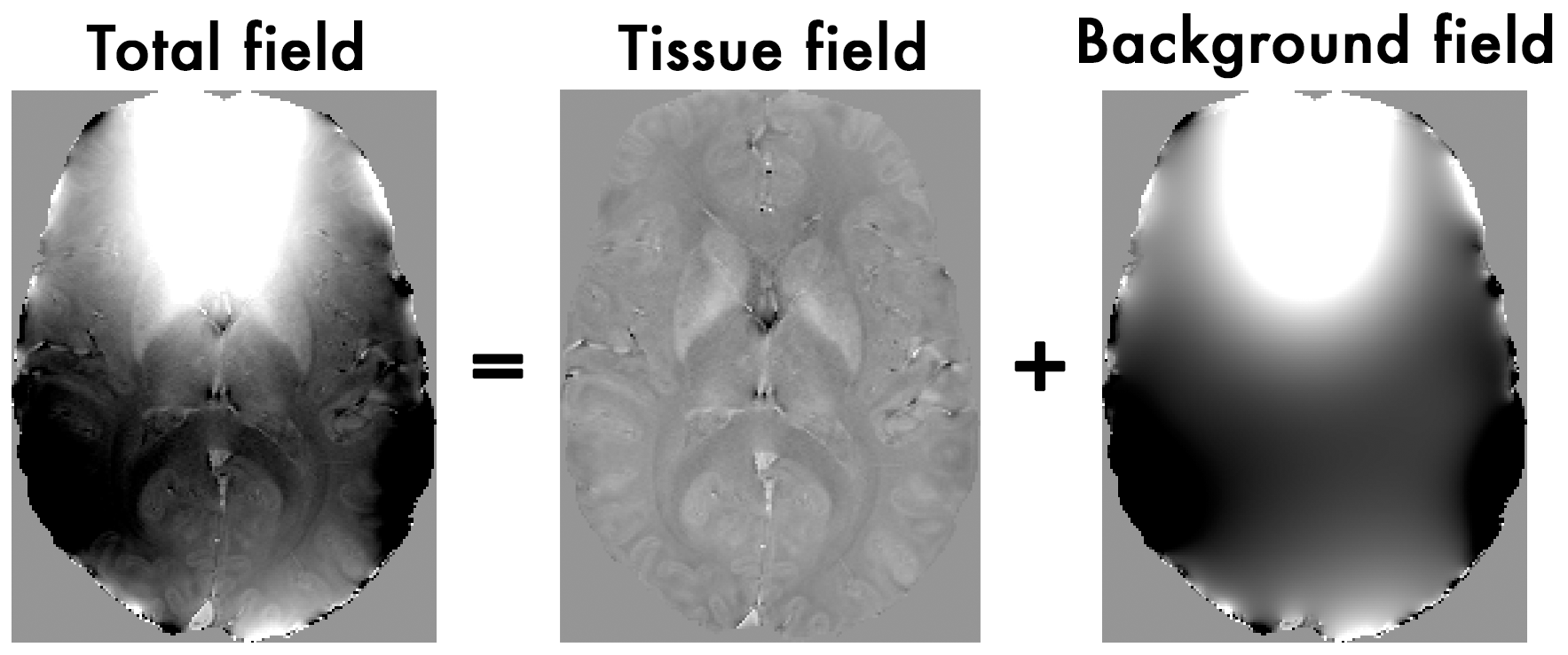
Figure 1: The total field we obtained from the last exercise is the summation of tissue and background magnetic fields. In order to compute the magnetic susceptibility of the brain tissue correctly, the background field contributions have to be removed before mapping the tissue susceptibilities.
SEPIA provides 7 methods to remove the background magnetic fields. Today we will use the so-called Sophisticated Harmonic Artifact Reduction for Phase (SHARP) algorithm to do this job.
Exercise 3.1
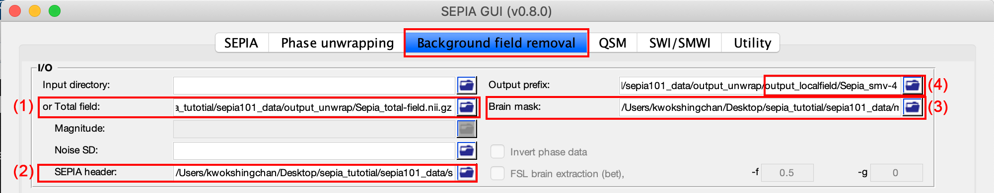
Go to the Background field removal tab. You will see two panels as in the Phase unwrapping tab.
In the I/O panel, specify the required files by using the  buttons:
or Total field: Sepia_total-field.nii.gz (in ~/sepia_tutorial/sepia_data/output_unwrap/),
SEPIA Header: Sepia_header.mat (in ~/sepia_tutorial/sepia_data/),
Brain mask mask.nii.gz (in ~/sepia_tutorial/sepia_data/),
Change the Output prefix to: ~/sepia_tutorial/sepia101_data/output_unwrap/output_localfield/Sepia_smv-4
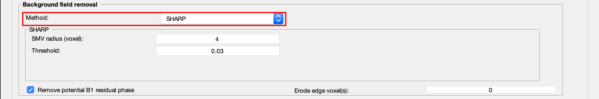
Second, in the Background field removal panel, change the Method to ‘SHARP’. You can have two parameters to adjust.
‘SMV radius (voxel)’: radius of a spherical mean value (SMV) kernel, in number of voxels
‘Threshold’: threshold used in Truncated SVD.
Press the Start button.
Again, when the process is finished, you will see the message: ‘Processing pipeline is completed!’.
Once the process is finished, you should be able to see the following output in the output directory (~/sepia_tutorial/sepia101_data/output_unwrap/output_localfield/)
Output data
Description
sepia_config.m
Automatic generated script by the GUI of SEPIA containing all user specified parameters
run_sepia.log
Event log file of the Matlab’s command window output
Sepia_smv-4_local-field.nii.gz
Local (tissue) field map in Hz
Sepia_smv-4_mask-qsm.nii.gz
Signal mask for QSM step
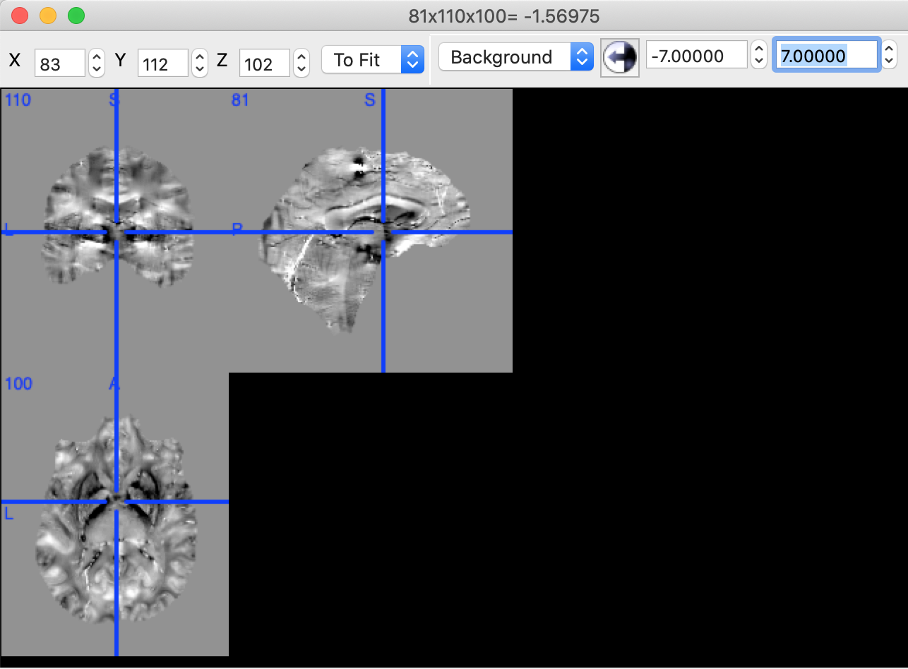
Open the local field map with any NIfTI image view (e.g.
FSLeyesormricron). Adjust the display window to ‘Min -7’ and ‘Max 7’.Note you can clearly see the contrast between grey and white matter, and veins and tissue now. Other structures as the globus pallidus, red nuclei and substantia nigra are visible… but not quite normal.
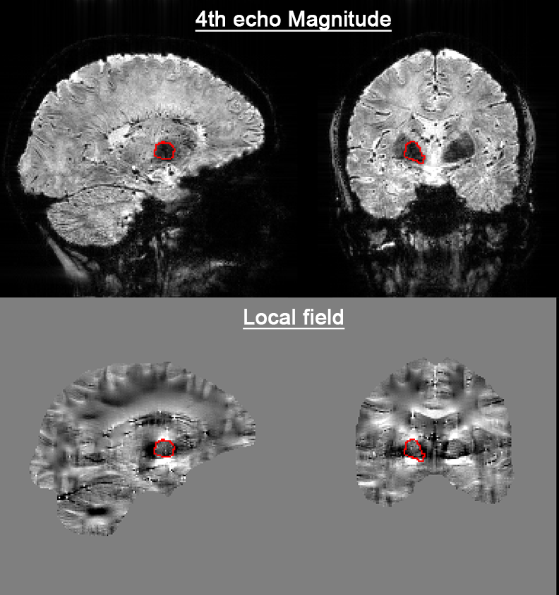
The figure below shows the last echo of magnitude data, where the globus pallidus is circled by red line, based on the image intensity, and the corresponding local field map. It is known that globus pallidus has a high iron content which can generate a strong induced magnetic field.
Can you guess the shape and sign of the magnetic properties of the globus palllidus?
You can close all the NIfTI viewers now.
Proceed to Exercise 4.
Exercise 3.2 (Advanced)
Note
If you still have enough time, follow the exercise below.
In this exercise, we will focus on the effect of using a different ‘SMV radius (voxel)’ value.
Change the Output prefix to: ~/sepia_tutorial/sepia101_data/output_unwrap/output_localfield/Sepia_smv-2
Set SMV radius (voxel) in the Background field removal panel to: 2
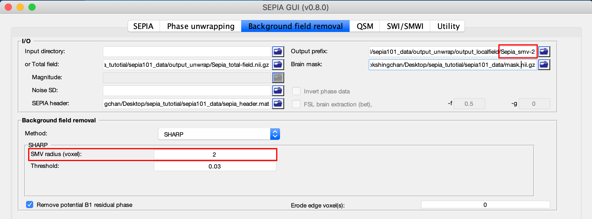
Press the Start button. Again, when the process is finished, you will see the message: ‘Processing pipeline is completed!’.
Try open Sepia_smv-2_local-field.nii.gz and Sepia_smv-4_local-field.nii.gz at the same time. Adjust the display window to ‘Min -7’ and ‘Max 7’ for both images. What differences can you see between the two results?
Proceed to Exercise 4.
Back to Exercise 2.