Exercise 4

Objectives

• Understanding QSM dipole inversion

• Gaining experience to use QSM algorithms

Data Required

Data	Description
Sepia_local-field.nii.gz	Local (tissue) field map in Hz , in ~/sepia_tutorial/sepia_data/output_unwrap/output_localfield/
Sepia_smv-4_mask-qsm.nii.gz	Signal mask for QSM step , in ~/sepia_tutorial/sepia_data/output_unwrap/output_localfield/
sepia_header.mat	contains important information such as the echo times (TE) and magnetic field strength (in Tesla), and orientation of the acquisition regarding the physical coordinates of the scanner. These are important to compute the magnetic susceptibility with the correct units and ensure the physical model is correct , in ~/sepia_tutorial/sepia_data/

Estimated time

About 15 min.

The Last Step

The last step of QSM processing is to deconvolute the local (tissue) field by the unit dipole field, such that the tissue magnetic susceptibility can be revealed. This can be described by:

(1)

where and are the Fourier and inverse Fourier transform operators.

This is the so-called dipole inversion of QSM, which is just the element-wise division between the Fourier transforms of the two images.

• Theory: Dipole Inversion

Sounds simple, isn’t it? Let’s try it out!

QSM: Dipole inversion

Move to the QSM tab of SEPIA.

Exercise 4.1

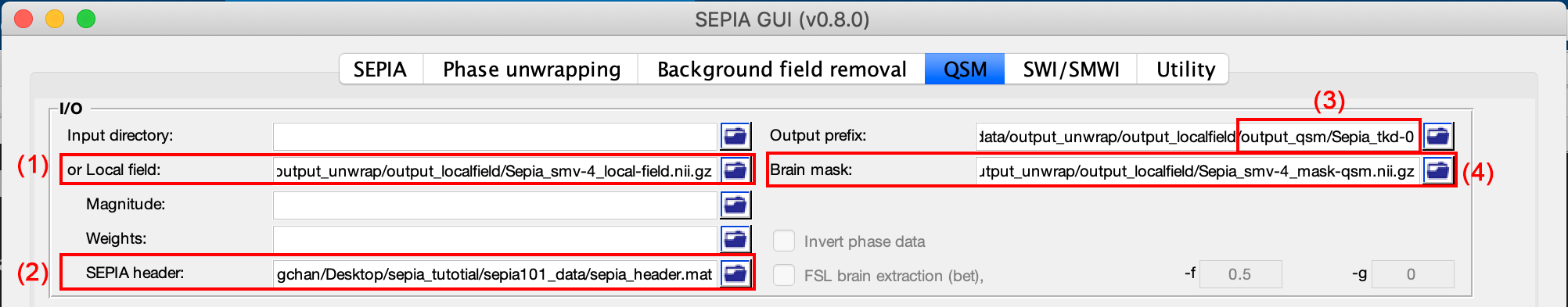
I/O panel:

1. Select the or Local field input: Sepia_smv-4_local-field.nii.gz (in ~/sepia_tutorial/sepia_data/output_unwrap/output_localfield/),

2. Select the SEPIA Header: Sepia_header.mat (in ~/sepia_tutorial/sepia_data/),

3. Change the Output prefix of the output to: ~/sepia_tutorial/sepia_data/output_unwrap/output_localfield/output_qsm/Sepia_tkd-0,

4. Select the Brain mask: Sepia_smv-4_mask-qsm.nii.gz (in ~/sepia_tutorial/sepia_data/output_unwrap/output_localfield/).

   Note

   An updated brain mask has to be used here because some edge voxels were excluded from the original brain mask in the last operation.

   

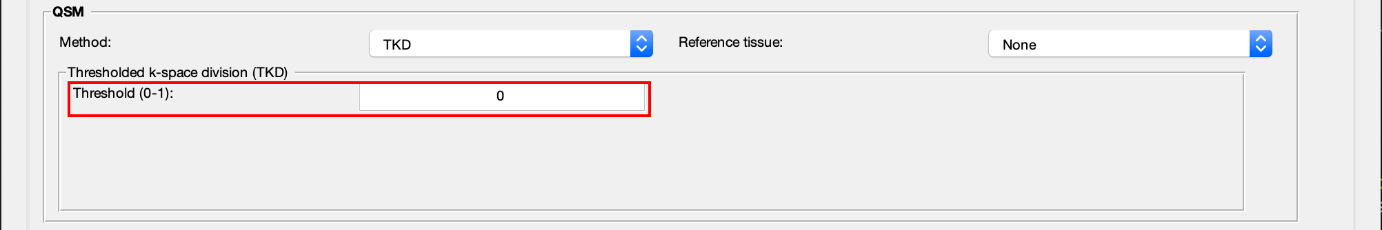
QSM panel:

5. To do exactly the operation as in Eq. (1), set the threshold of the TKD algorithm to ‘0’ and press Start.

   

6. Check the result Sepia_tkd-0_QSM.nii.gz in the output directory. Set the display window to ‘Min. -0.1’ and ‘Max. 0.1’ (ppm). Does it look like the QSM map as we expected?

• Answer: Exercise 4.1

Exercise 4.2

To avoid the previous QSM map we can increase the threshold value of the TKD.

1. Change the Output orefix to: ~/sepia_tutorial/sepia_data/output_unwrap/output_localfield/output_qsm/Sepia_tkd-0p15.

2. Change the threshold of the TKD algorithm to 0.15 and press Start.

3. Check the result Sepia_tkd-0p15_QSM.nii.gz in the output directory. Display it along with the Sepia_tkd-0_QSM.nii.gz. Set the display window to ‘Min. -0.1’ and ‘Max. 0.1’ (ppm). Do you see any improvement?

• Answer: Exercise 4.2

Congratulations! You have finished all the exercises in this tutorial. If you still have time left, finish the advanced exercises or experiment with different QSM methods/methods’ parameters.

Advanced Exercise 4.3

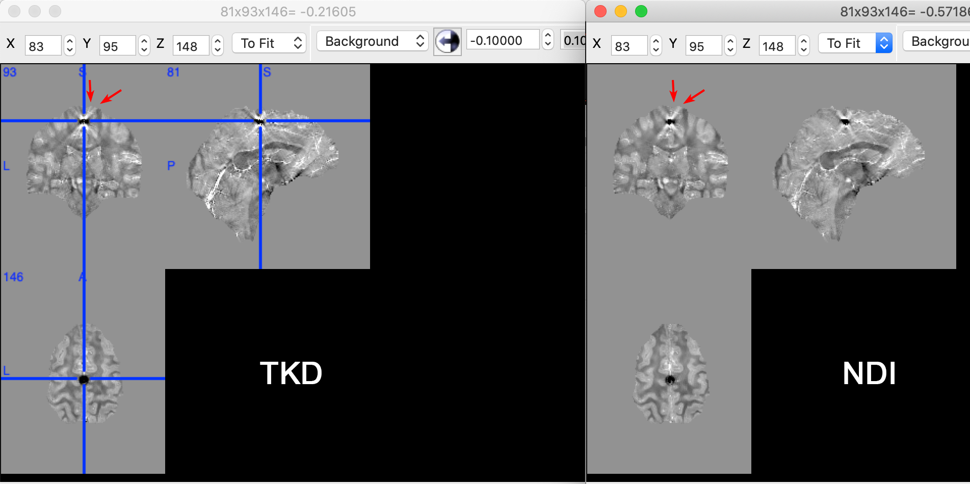
To further improve the quality of the QSM map, some methods, such as non-linear dipole inversion (NDI), incorporate additional information, e.g. SNR weighting, with advanced processing algorithm.

1. Select the Weights input: Sepia_weights.nii.gz (in ~/sepia_tutorial/sepia_data/output_unwrap/),

2. Change the Output prefix to: ~/qsm_tutorial/data/output_qsm/Sepia_ndi.

3. Change the QSM method to ‘NDI’ and keep the default setting. Press Start. It will take about a few minutes to finish.

Open the result Sepia_tkd-0p15_QSM.nii.gz and Sepia_ndi_QSM.nii.gz togther. If you are using mricron, go to location [83,95,148], which is the location of calcification in the phantom data. Can you see that the NDI’s result has less artefact?

Back to Exercise 3.