Exercise 4
Objectives
Understanding QSM dipole inversion
Comparing a QSM reconstruction and an R2* map and find the relevant deep gray matter nuclei visualizes.
Data Required
a 3D recontructed R2* map (Sepia_R2starmap.nii.gz in the Exercise 2 output directory)
a 3D recontructed QSM map (Sepia_Chimap.nii.gz in the Exercise 3 output directory)
a 3D local field image (Sepia_localfield.nii.gz in the Exercise 3 output directory)
a 3D refined brain mask (Sepia_mask_QSM.nii.gz in the Exercise 3 output directory)
a SEPIA header (Sepia_header.mat in the input data directory)
Estimated time
About 15 min.
The Last Step
The last step of QSM processing is to deconvolute the local (tissue) field by the unit dipole field, ‘d’, such that the tissue magnetic susceptibility can be revealed. This can be described by:
(1)![\chi = F^{-1}[\frac{F(Tissue field)}{F(d)}]](../../_images/math/1c2dd8d0b32e001e749b6e2ea213cf38cfb1f80c.png)
where  and
and  are the Fourier and inverse Fourier transform operators.
This is the so-called dipole inversion of QSM, which is just the element-wise division between the Fourier transforms of the two images. It can also be seen as a deblurring process.
One extra QSM reconstruction
Move to the QSM tab of SEPIA.
In the IO panel, we will now simply select the data required to perform the QSM step, starting from the previously pre-processed data.
Select the Local field: ~/QuantitativeTutorial/outputQSM/Sepia_localfield.nii.gz
Select the weights: ~/QuantitativeTutorial/outputQSM/Sepia_weights.nii.gz
Select the Brain Mask: ~/QuantitativeTutorial/outputQSM/Sepia_mask_QSM.nii.gz
Select the SEPIA header: ~/QuantitativeTutorial/data/sepia_header.mat
Change the Output basename to: ~/QuantitativeTutorial/outputQSM/SepiaSTAR
Note
1: The various preprocessing steps will erode the brain mask, resulting in a final brain mask that is significantly tighter.
Note
2: More advanced methods of QSM benefit from knowing about the confidence you have on your measured fieldmap, that information is embedded on ‘weights’
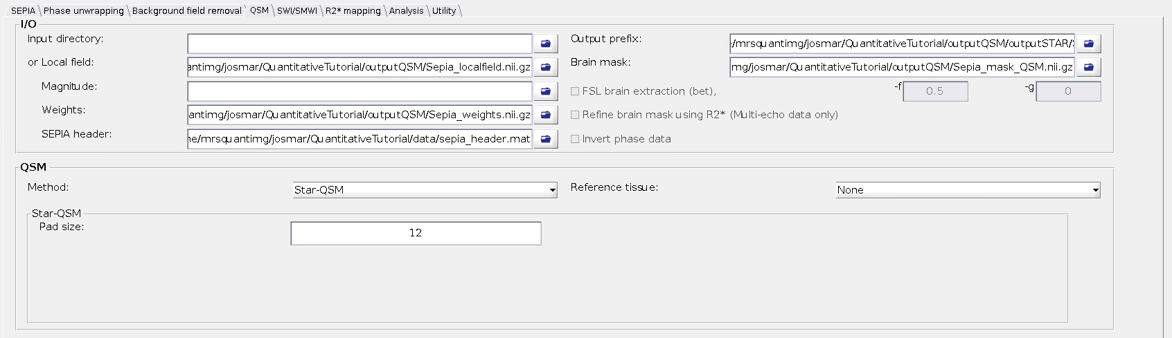
In the QSM panel you will now choose the STAR method (Wei et al, NMR in Biomed, 2015).
Press start on the SEPIA window and continue the exercise.
In Exercise 2, you already had a chance to see many iron rich strucures throught out the brain.
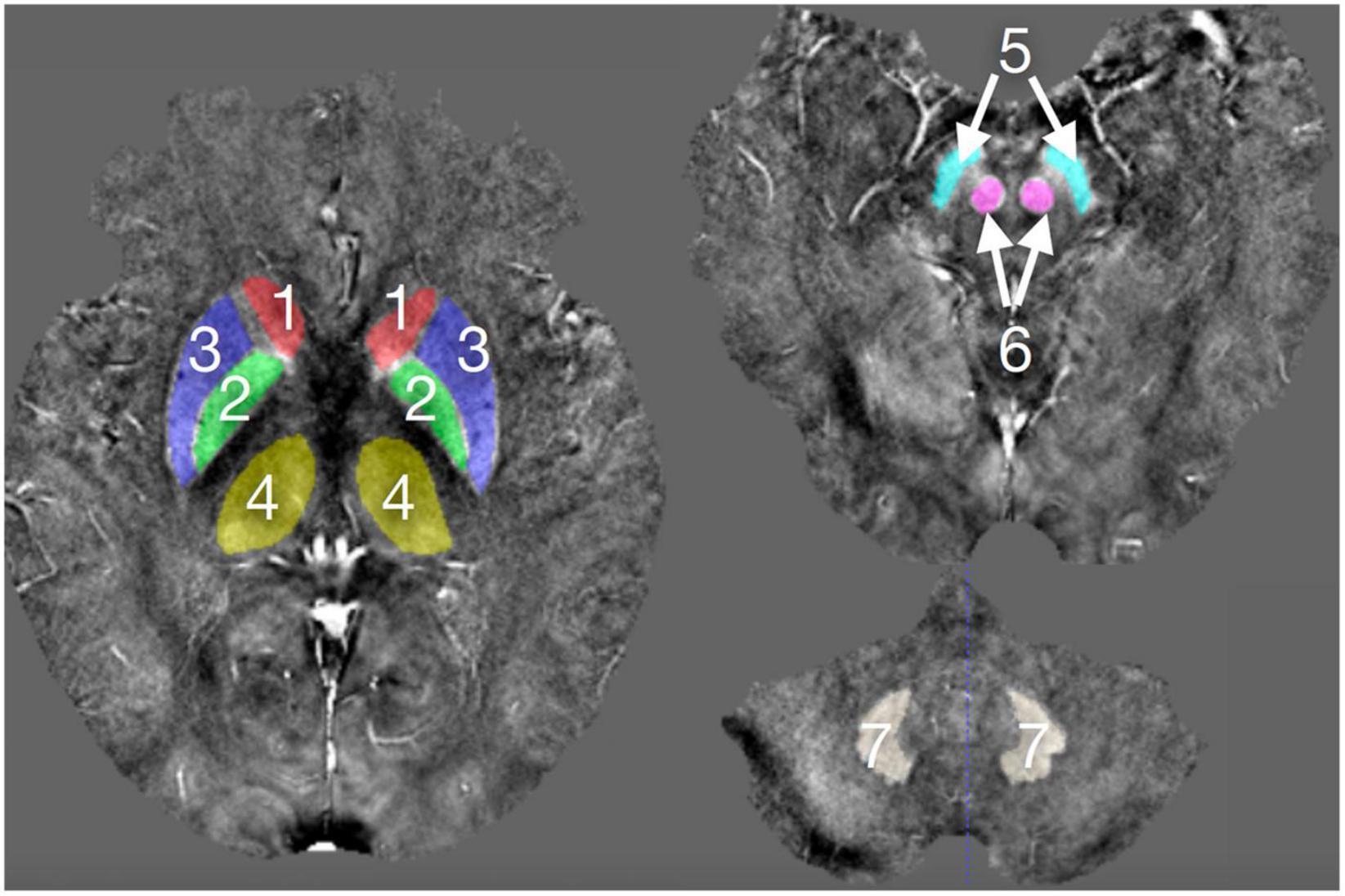
1, Caudate Nucleus; 2, Globus pallidus; 3, Putamen, 4, Thalamus; 5, Substantia Nigra; 6, Red Nucleus; 7, Dentate Nucleus; Figure from Chai et al, Front. Neurosci., 2022
Return to the terminal and type:
cd ~/QuantitativeTutorial
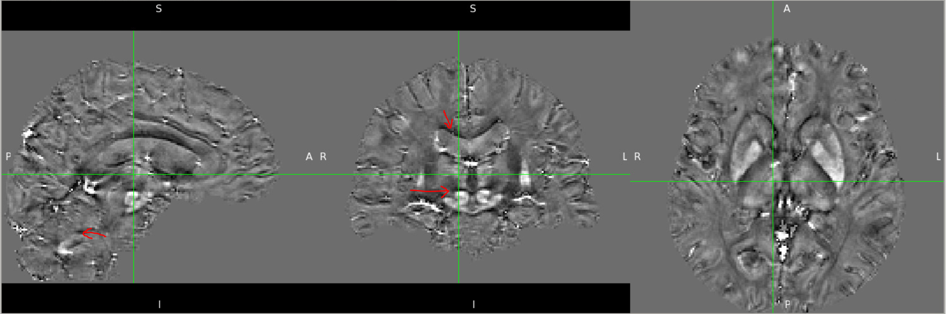
``fsleyes outputR2star/Sepia_R2starmap.nii.gz -dr 0 50 outputQSM/SepiaSTAR_Chimap.nii.gz -dr -0.15 0.2 outputQSM/Sepia_Chimap.nii.gz -dr -0.15 0.2 outputQSM/Sepia_localfield.nii.gz -dr -5 5 ``
As the top layer you will have the local field map that you have already seen on the previous exercise.
While many of the deep gray matter regions mentioned above are clear discernible, with very sharp edges, the intensity inside the regions is not very different than that of White Matter.
If you now remove the visibility of this first layer you will be able to see the reconstructed QSM (TKD) where these ROIs are now visible and have a strong positive contrast (meaning they have paramagnetic properties - rich in iron).
If you now vary between the visibility of the two QSM reconstructions you will note that SepiaSTAR_Chimap has less deconvolution artifacts and that the edges of Iron rich structures have less artifacts on the edges.
Note
3: The level of paramagnetism (brightness of the different deep gray matter structures) is also not exactly the same in the two maps… While this gets more stable as more advanced methods are used, one should avoid comparing QSM values obtained from different reconstruction pipelines!
Finally you can appreciate the difference between the R2* and Star QSM recosntruction. Points to note:
the reduced mask size associated with the QSM reconstruction;
while the R2* map has a strong tissue CSF contrast, this is vanished in the QSM showing that the magnetic properties of most brain tissue is comparable
appreciate the increased visibility of the Substantia Nigra and Dentate Nucleus on the QSM map.
Congratulations! You have finished all the exercises in this tutorial.
If you still have time left, experiment with different QSM methods/parameters or move to the next exercise that will show you how to get Synthetic images out of some of these images and maps.
Advanced Exercise, open the config files of the exercises 3 and 4 in the editor and create a new matlab script file MyQSMrecon.m. In this file you can create a script that generates a truncated k-space division QSM map with a threshold of 0.0001.
Run the script from the Matlab command window and apreciate on FSLeyes a terrible but very accurate reconstruction!
Back to fmritoolkit2023-exercise3. Proceed to Exercise 5.