Exercise 3

Objectives

• Understanding QSM works

• Fine-tuning method parameters to improve the QSM reconstruction

Estimated time

About 15 min.

Data Required

• a 4D raw phase data (phase.nii.gz in the input directory)

• a 4D raw magnitude data (mag.nii.gz in the input directory)

• a 3D raw mask data (mask.nii.gz in the input directory)

• a SEPIA header (Sepia_header.mat in the input directory)

Performing a full QSM reconstruction

While Sepia allows to do perform the three steps of the QSM pocessing separatily (using the 2nd, 3rd and 4th tab respectively) here, for the interest of time, we will to it in one go.

You can see four sub-panels under the SEPIA tab:

• the I/O panel is for specifying data input and output;

• the Total field recovery and phase unwrapping panel is for selecting phase unwrapping and total field estimation algorithms

• the Background Field Removal (BFR) panel is for selecting the BFR algorithms that will deliver the tissue specific field variations

• the QSM panel allows you to choose the QSM algorithms and respective parameters

Tip

SEPIA supports two types of data input. If your data follows the SEPIA naming structure, you can select the directory containing all the input data as your input in the first row of I/O panel. Alternatively, you can specify the input files separately by following the instruction of the second row of the I/O panel.

Here, for educational purposes, we will explicitely introduce the input data

In the I/O panel:

1. Select the Input Phase: ~/QuantitativeTutorial/data/phase.nii.gz

2. Select the Magnitude: ~/QuantitativeTutorial/data/mag.nii.gz

3. Select the Brain Mask: ~/QuantitativeTutorial/data/mask.nii.gz

4. Select the SEPIA header: ~/QuantitativeTutorial/data/sepia_header.mat

5. Change the Output basename to: ~/QuantitativeTutorial/outputQSM/Sepia

6. Turn on Refine brain mask

While earlier we mentioned that it was the phase data that was needed to compute QSM, in practice you also need the magnitude to learn how trustworhy your phase data is.

For the purpose of this tutorial we will broadly follow the current QSM harmonization settings for both the total field computation and background field removal, but select a more time efficient reconstruction for the last step (QSM).

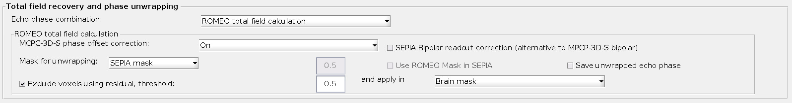
In the Total field recovery and phase unwrapping panel:

1. Change the Echo phase combination method to ‘ROMEO total field calculation’

2. Change the MCPC-3D-S phase offset method to ‘On’

3. Change the Mask for unwrapping method to ‘SEPIA mask’.

4. Select Exclude voxels using Residual and apply it on ‘Brain mask’.

   

Note

Alternatively, Optimum weights and MEDI nonlinear fit echo phase combination combined with either SEGUE or ROMEO phase unwrapping can perform comparably but can be more time consuming.

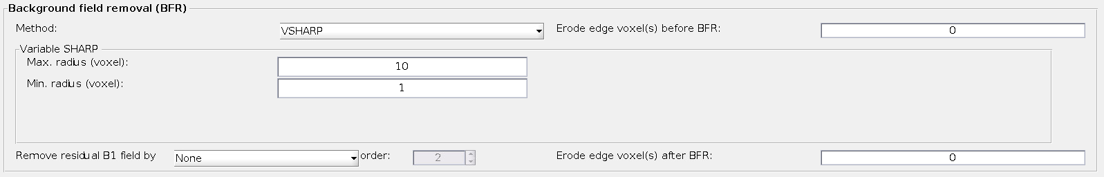
In the Background field removal panel, the ‘LBV’ method is shown by default. While this would be an acceptable option. In this tutorial we will choose the more robust to noise option VSHARP

• ‘Erode edge voxel before BFR’: 0.

• ‘Max. radius’: 10.

• ‘Min. radius’: 1.

• ‘Remove Residual’: ‘None’.

  

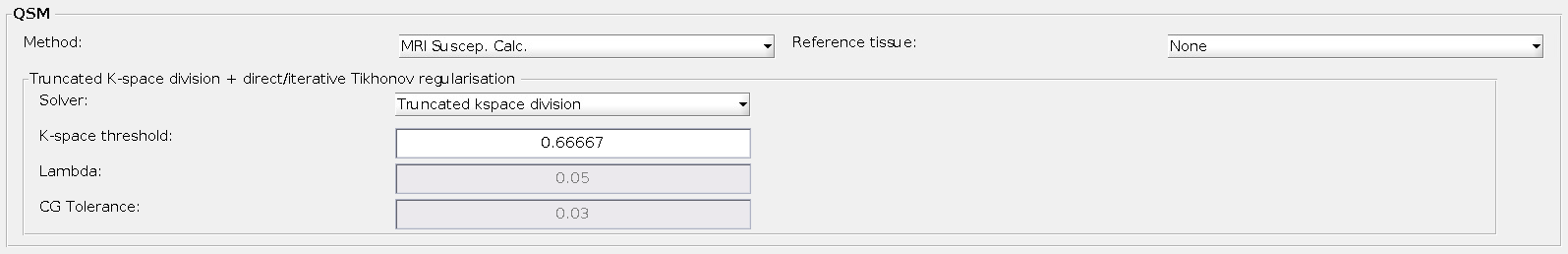
In the QSM pannel there are various methods that have been implemented by different teams around the world.

There are :

• AI GPU enabled reconstructions (xQSM, LPCNN, QSM+);

• Iterative reconstructions;

• Direct or Close form solutions;

The first class requires GPU hardware, the second often requires some parameter tunning and can be very time consuming. The thrid class, while simplistic, is very time and memory efficient. In this tutorial it is suggested you:

• Select the Method the ‘MRI Suscep. Calc.’ (Univerity College of London Toolbox);

• Select solver ‘Truncated kspace division’;

• Use the suggested provide K-space Threshold of 0.66 (Schwezer et al, MRM, 2012).

  

Press on the start button. On the command window some text will appear reflecting the progress of your pipeline as well as some of the choices you have made. Wait until: ‘Processing pipeline is completed!’.

Tip

All the output messages of SEPIA will be displayed on the Matlab command window. Make sure you check the command window before clicking the Start button again with a new set of parameters you might want to try! You can in the mean while also open the ‘Sepia_config.m’ in the ‘outputQSM’ directory. You will see that all the parameters you chose are present in that file: great for reproducible science and for future scripting!

Check the output (should be in ~/QuantitativeTutorial/outputQSM/). In the terminal you can do this by typing

ls -alt ~/QuantitativeTutorial/outputQSM

which will give a list of the files on your output directory ordered by creation time. You should recognise here the order of the the full QSM pipeline.

You will now visualise the main outputs of the total field calculation, background field removal and compare them to the original phase data. Type on the terminal:

cd ~/QuantitativeTutorial/outputQSM fsleyes data/phase.nii.gz outputQSM/Sepia_fieldmap.nii.gz -dr -200 200 outputQSM/Sepia_localfield.nii.gz -dr -200 200

You should see the following viewer with three layers and the different images will already have the predefined color display ranges.

The first dataset is the standard phase images (units in radians). You can make the different layers visible by clicking on the eye next to the dataset name at the bottom left of the fsl window. If you have selected the phase dataset you can use the volume counter to see the different echo times In the second map (already in fequency units, Hz) you have the computed total field. This has no phase wraps and contains all the information present across all the echo times. This was computed using the unwrapped phase images at the different echo times using the knowlege and taking into account of the SNR of each echo:

Finally, as you click and unclick the third layer, you will see the that the local field only conserves high-spatial frequency features and has very low amplitude values

1. Adjust the display window to ‘Min -10’ and ‘Max 10’ for the localfield and you will see a lot of relevant anatomical information that was hidden bellow the background field

2. Set location as [120 112 49]. Can you see a spherical structure emanating a magnetic field? welcome to the red nucleus.

3. Use shortcut Crtl+O in the FSLeyes to add mean_head.nii.gz to the displayed local field maps (in the data directory).

4. Check/Uncheck the ‘Visibility’ button to turn on/off of the mean magnitude image.

5. It is known that there is a high concentration of iron deposition in the red nucleus (also in the globus pallidus [144 131 60]). This generates a strong secondary magnetic field that results in an enhancement of the edges of this structures.

The frequency map ìnitially computed contains magnetic fields generated by not only the brain tissue but also the scanner hardware imperfection and fields generated at air/tissue interfaces, where the susceptibility differences are one order of magnitude greater than inside the brain. Therefore, we have to remove the non-tissue field, or background field, contributions before computing the susceptibility map.

• One more step before computing QSM but why?

You can close all the FSLView window(s) now.

Proceed to fmritoolkit2025-exercise4.

Back to Exercise 2.