Exercise 1

Objectives

• Understanding the data required for QSM and R2*

• Understanding why we need to pre-process the phase data before mapping the magnetic susceptibility

Data Required

• a 4D raw phase data (phase.nii.gz in the input directory)

• a 4D raw magnitude data (mag.nii.gz in the input directory)

• a 3D brain mask (mask.nii.gz in the input directory)

• JSON files generated by data conversion software (all .json in the input directory)

if data has not already been made available by the course organizer, it can be downloaded from the following zenodo collection 10.5281/zenodo.8340358

Estimated time

About 15 min.

Understanding multi-echo GRE data

If using the Donders HPC, start an interactive session with increased memory by typing in the command in a terminal (you will use this terminal both to visualize data using fsleyes and to run MATLAB/SEPIA)

srun --x11  --time=21:00:00 --mem=20gb --pty bash -i

Go to the exercise directory which is located in ~/QuantitativeTutorial/.

You can use the following command in the terminal:

cd ~/QuantitativeTutorial/

Note

Here we assume your tutorial directory is in the home directory ‘~/’. If not, replace ‘~/’ with the path containing the folder ‘QuantitativeTutorial’.

To view the content of the directory use the command: ls

You will see one folder in the directory.

• data - contains the multi-echo gradient echo images we will work on.

Go to the data directory using cd data and have a look of the content inside the folder ls

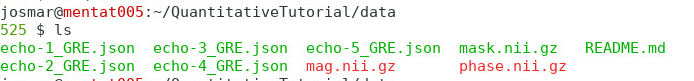
You should see three NIfTI images (.nii.gz) and a few JSON files (.json) in the directory:

• The NIfTI files mag.nii.gz and phase.nii.gz contain the magnitude and the phase data acquired with a multi-echo gradient echo sequence.

  Both images are 4D datasets, with the first 3 dimensions being spatial (i.e. the brain volume in x,y and z) and ** the echo time in the 4th dimension**.

• The NIfTI file mask.nii.gz contains a precomputed 3D brain mask

• The JSON files contain important information such as the echo times (TE) and magnetic field strength (in Tesla), orientation of the acquisition in respect to the physical coordinates of the scanner. These are essential parameteres to correctly define our magnetic dipole in the image space and compute the magnetic susceptibility, ensuring that the physical model is correct!

Magnitude images

1. Take a look at the magnitude images. You can do this byusing an image viewer such as FSLeyes. Type in the terminal:

   fsleyes mag.nii.gz &

   Tip

   The ‘&’ character will enable the viewer running in the background so you can still work with the current section in the terminal.

   Note

   Due to the file size, it can be better to view the images with FSLView (fslview_deprecated) instead of FSLeyes (fsleyes).

2. Adjust the display window to ‘Min 0’ and ‘Max 600000’.

3. Click the movie button or scroll through the 4th dimention to see how the brain contrast changes with respect to the echo time.

   

4. Click the movie button again to stop the movie. Press Ctrl+3 to see the plot of signal evolution at different brain tissues over time.

5. Select a few data points in the brain (e.g. Globus pallidus [108, 127, 62], white matter [89, 94, 62] and CSF [110 89, 62]), how do you describe the signal change with respect to the echo time? An exponential decay is not always quite obvious, but that is what we will assume.

6. Go back to the terminal. Compute the mean magnitude image in time:

   fslmaths mag.nii.gz -Tmean mean_head.nii.gz

   This image will be used in Exercise 3.

Phase images

Phase images are traditionaly discarded, yet they are essential to compute a magnetic susceptibility map. For QSM multi-echo gradient-echo images are usually used to obtain this phase images that encode the local magnetic field strength.

• Theory: MR Phase

1. Look at the phase images:

   fsleyes phase.nii.gz &

   The phase images look different compared to the magnitude images and with the current display window it is hard to see any contrast in brain tissues.

2. Adjust the display window to ‘Min. -3’ and ‘Max. 3’ and go through different slices. You should be able to identify some brain structures (e.g. at slice 61).

   

Based on Eq. (1), it is expected the phase increases/decreases monotonically. In other words, we should observe the phase contrasts become higher in the later echoes (i.e. bright → brighter; dark → darker).

(1)

1. Click the movie button or scroll through the volumes to see the phase development over time. Can you make this observation?

2. Stop the movie and press Ctrl+3 to see the phase accumulation at those problematic regions (e.g. near the prefrontal cortex [126,161,62] ). Is the phase increasing linearly? Can you identify the cause of the problem?

   • A. Somebody screwed up the acquisition
   • B. The subject moved during the scan
   • C. The phase is bounded to certain values

In order to estimate the frequency shift correctly using Eq. (1), this phase problem has to be addressed which is called phase unwrapping.

To unwrap the phase and to map back to the correct values, SEPIA provides several algorithms to do the job.

You can close all the FSLeyes window(s) now.

Proceed to Exercise 2.