Exercise 2
Objectives
Gaining experience in using SEPIA
Understanding how to perform phase unwrapping
Data Required
a 4D raw phase data (phase.nii.gz in the input directory)
a 4D raw magnitude data (mag.nii.gz in the input directory)
JSON files generated by data conversion software (all .json in the input directory)
Estimated time
About 20 min.
SEPIA
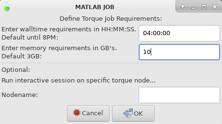
SEPIA is a pipeline tool to process phase images in Matlab. To use SEPIA, please open a Matlab application in the cluster by typing:
matlab2016b,
click OK, leave the runtime as default and specify the memory requirement as 10 (GB).
Once Matlab is open, go to the tutorial directory and add the SEPIA home directory to the Matlab Path:
addpath('~/qsm_tutorial/sepia/');
Note
The copy of SEPIA you have in the tutorial directory already includes all the external toolboxes required. If you want to know how to set up SEPIA from scratch for your research purposes, you can refer to Download.
Now, go the data directory in the Matlab command window and start sepia:
cd ~/qsm_tutorial/data
sepia
A graphical user interface (GUI) should be pop up.

The first tab in SEPIA provides a one-step application to process QSM from the raw phase data to a magnetic susceptibility map.
Alternatively, we can break down the processing pipeline into several steps and SEPIA also supports this approach.
Create a SEPIA header
Before using the SEPIA, create a header file that contains all essential information regarding the data acquisition (magnetic field, resolution, echo time).
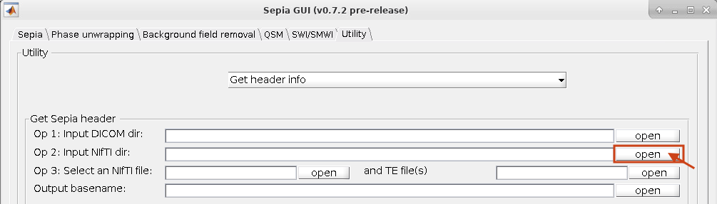
Select the Utility tab and then select Get header info in the drop-down menu. This function provides several ways to extract the header information from different files.
With all the NifTI images and JSON files stored in the same place, we can use ‘Op 2’ routine:
Click Open next to ‘Op 2’
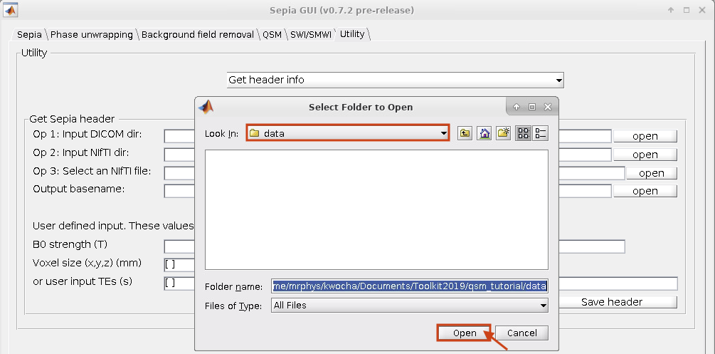
Select ~/qsm_tutorial/data as the input (The dialog box will show the current directory in Matlab).
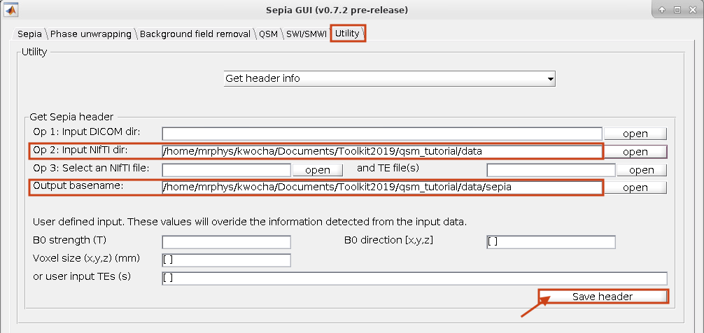
Click Save header to save the file.
The process is done when you see the message ‘SEPIA header is saved!’ in the command window. You should see a new file is generated in the input directory.
Your setting should be like:
Phase Unwrapping and Total Field Computation
To correct the wrapped phase in the raw images, go the Phase unwrapping tab (next to Sepia tab).
You will see two panels under the tab: the I/O panel is for specifying data input and output and the Total field recovery and phase unwrapping panel is for selecting phase unwrapping and true phase estimation algorithms.
Tip
SEPIA supports two types of data input. If your data follows the SEPIA naming structure, you can select the directory containing all the input data as your input in the first row of I/O panel. Alternatively, you can specify the input files separately by following the instruction of the second row of the I/O panel.
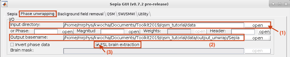
In the I/O panel:
Select the Input directory: ~/qsm_tutorial/data
Change the Output basename to: ~/qsm_tutorial/data/output_unwrap/Sepia
Check the FSL brain extraction
It is essential to have a brain mask to produce a high-quality QSM map.
In the Total field recovery and phase unwrapping panel:
Keep the Echo phase combination method as ‘Optimum weights’
Change the Phase unwrapping method to ‘Laplacian STI suite’.
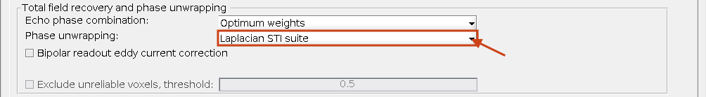
Then click the Start button.
You should now see some messages displayed in the Matlab’s command window. These messages give you the general information of your input data and the overview of the selected method(s). Once the process finishes (~3min), you will see the message
‘Processing pipeline is completed!’.
Tip
All the output messages of SEPIA will be displayed on the Matlab command window. Make sure you check the command window before clicking the Start button again!
Check the output (should be in ~/qsm_tutorial/data/output_unwrap/), in the terminal type:
fslview_deprecated Sepia_unwrapped-phase.nii.gz
fslview_deprecated Sepia_total-field.nii.gz
The first dataset is the unwrapped phase images (unit in radian). Play the movie to see the phase development. All the zebra-line pattern and phase jumps are gone in the later echo images (e.g. near the prefrontal cortex [113 195 65]).
Note
Besides the ability of phase unwrapping, Laplacian based operation removes some harmonic fields. Therefore, the phase values in the unwrapped phase map cannot be comparable to the raw wrapped phase.
The second dataset corresponds to the frequency (Hz) map which was computed using the unwrapped phase images at the different echo times illustrated in Eq. (1):
(1)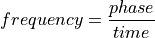
The latter is the result needed in the next exercise.
You can close all the FSLView window(s) now.
Proceed to Exercise 3.
Back to Exercise 1.