Exercise 1

Objectives

• Understanding the data required for QSM

• Understanding why we need to correct the phase data before mapping the magnetic susceptibility

Data Required

• a 4D raw phase data (phase.nii.gz in the input directory)

• a 4D raw magnitude data (mag.nii.gz in the input directory)

• JSON files generated by data conversion software (all .json in the input directory)

Estimated time

About 15 min.

Understanding multi-echo GRE data

To compute a magnetic susceptibility map, multi-echo gradient-echo images are usually used because it can provide phase images.

• Theory: MR Phase

Go to the exercise directory which is located in ~/qsm_tutorial/.

You can use the following command in the terminal:

cd ~/qsm_tutorial/

Note

Here we assume your tutorial directory is in the home directory ‘~/’. If not, replace ‘~/’ with the path containing the folder ‘qsm_tutorial’.

To view the content of the directory use the command: ls

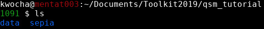
You will see there are two folders in the directory.

• sepia - contains the software we will use throughout this tutorial;

• data - contains the multi-echo gradient echo images we will work on.

Go to the data directory using cd data and have a look of the content inside the folder ls

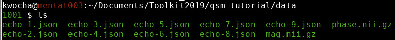
You should see two NIfTI images (.nii.gz) and a few JSON files (.json) in the directory:

• The NIfTI files mag.nii.gz and phase.nii.gz contain the magnitude and the phase data acquired with a multi-echo gradient echo sequence.

  Both images are 4D datasets, with the first 3 dimensions containing spatial information (i.e. the image of the brain) and echo time in the 4th dimension.

• The JSON files contain important information such as the echo times (TE) and magnetic field strength (in Tesla), and orientation of the acquisition regarding the physical coordinates of the scanner. These are important to compute the magnetic susceptibility with the correct units and ensure the physical model is correct.

Magnitude images

1. Take a look at the magnitude images. You can do this by calling the image viewer FSLView in the terminal:

   fslview_deprecated mag.nii.gz &

   Tip

   The ‘&’ character will enable the viewer running in the background so you can still work with the current section in the terminal.

   Note

   Due to the file size, it is better to view the images with FSLView instead of FSLeyes.

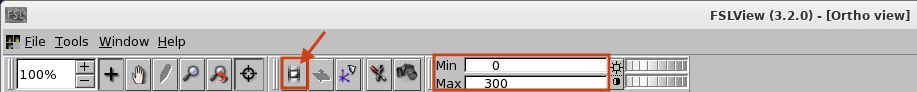
2. Adjust the display window to ‘Min 0’ and ‘Max 300’.

3. Click the movie button to see how the brain contrast changes with respect to the echo time (time between echoes = 4ms).

   

4. Click the movie button again to stop the movie. Press Ctrl+T to see the plot of signal evolution at different brain tissues over time.

5. Select a few data points in the brain (e.g. caudate nucleus [98 169 87], white matter [143 106 92], and cortical grey matter [159 190 77]), how do you describe the signal change with respect to the echo time in general?

   • Check Your Progress 1

6. Go back to the terminal. Compute the mean magnitude image in time:

   fslmaths mag.nii.gz -Tmean mean_head.nii.gz

   This image will be used in Exercise 3.

Phase images

1. Look at the phase images:

   fslview_deprecated phase.nii.gz &

   The phase images look different compared to the magnitude images and with the current display window it is hard to see any contrast in brain tissues.

2. Adjust the display window to ‘Min. -3.14’ and ‘Max. -1’ and go through different slices. You should be able to identify some brain structures (e.g. at slice 82).

   

3. Change the window back to ‘Min. -3.14’ and ‘Max. 3.14’.

Based on Eq. (1), it is expected the phase increases/decreases monotonically. In other words, we should observe the phase contrasts become higher in the later echoes (i.e. bright → brighter; dark → darker).

(1)

1. Click the movie button to see the phase development over time. Can you make this observation?

   • Check Your Progress 2

2. Stop the movie and press Ctrl+T to see the phase accumulation at those problematic regions (e.g. near the prefrontal cortex [113 195 65]). Can you identify the cause of the problem?

   • A. Somebody screwed up the acquisition
   • B. The subject moved during the scan
   • C. The phase is bounded to certain values
   • D. Fast switching gradient introduced extra phase
   • E. I don’t know. I’m here to learn some fMRI analysis so just show me the answer

In order to estimate the frequency shift correctly using Eq. (1), this phase problem has to be addressed which is called phase unwrapping.

To unwrap the phase and to map back to the correct values, SEPIA provides several algorithms to do the job, and this is what we are going to do in the next exercise.

You can close all the FSLView window(s) now.

Proceed to Exercise 2.