Exercise 4
Objectives
Understanding QSM dipole inversion
Gaining experience to use QSM algorithms
Data Required
a 3D local field image (Sepia_peel-4_local-field.nii.gz in the previous exercise output directory)
a 3D refined brain mask (Sepia_peel-4_mask-qsm.nii.gz in the previous exercise output directory)
a SEPIA header (Sepia_header.mat in the input directory)
Estimated time
About 15 min.
The Last Step
The last step of QSM processing is to deconvolute the local (tissue) field by the unit dipole field, such that the tissue magnetic susceptibility can be revealed. This can be described by:
(1)![\chi = F^{-1}[\frac{F(Tissue field)}{F(d)}]](../../_images/math/1c2dd8d0b32e001e749b6e2ea213cf38cfb1f80c.png)
where  and
and  are the Fourier and inverse Fourier transform operators.
This is the so-called dipole inversion of QSM, which is just the element-wise division between the Fourier transforms of the two images.
Sounds simple, isn’t it? Let’s try it out!
QSM: Dipole inversion
Move to the QSM tab of SEPIA.
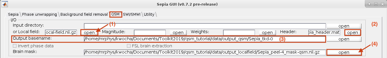
Exercise 4.1
I/O panel:
Select the Local field input: Sepia_peel-4_local-field.nii.gz (from the previous exercise output directory),
Select the Header: Sepia_header.mat,
Change the Output basename of the output to: ~/qsm_tutorial/data/output_qsm/Sepia_tkd-0,
Select the Brain mask: Sepia_peel-4_mask-qsm.nii.gz (from the previous exercise output directory).
Note
An updated brain mask has to be used here because some edges were excluded from the original brain mask in the last operation.
QSM panel:
To do exactly the operation as in Eq. (1), set the threshold of the TKD algorithm to ‘0’ and press Start.

Check the result Sepia_tkd-0_QSM.nii.gz in the output directory. Set the display window to ‘Min. -0.2’ and ‘Max. 0.2’ (ppm). Does it look like the QSM map as we expected?
Exercise 4.2
To avoid the previous QSM map we can increase the threshold of the TKD.
Change the Output basename to: ~/qsm_tutorial/data/output_qsm/Sepia_tkd-0p15.
Change the threshold of the TKD algorithm to 0.15 and press Start.
Check the result Sepia_tkd-0p15_QSM.nii.gz in the output directory. Display it along with the Sepia_tkd-0_QSM.nii.gz in FSLView. Do you see any improvement?
Compare the location on the tissue edges (e.g. [133 155 81]) in this QSM map with what you can see in the mean magnitude image mean_head.nii.gz. Do the edges match between the two data now?
Congratulations! You have finished all the exercises in this tutorial. If you still have time left, finish the advanced exercises or experiment with different QSM methods/methods’ parameters.
Advanced Exercise 4.3
To further improve the quality of the QSM map, some methods, such as Star-QSM, incorporate additional information, e.g. smoothness of the QSM map, during the QSM dipole inversion.
Change the Output basename to: ~/qsm_tutorial/data/output_qsm/Sepia_star-qsm.
Change the QSM method to ‘Star-QSM’ and press Start. It will take about 2 mins to finish.
It is difficult to see the differences between the two QSM maps with the naked eyes. Subtract the two maps so that you can see the differences:
fslmaths Sepia_tkd-0p15_QSM.nii.gz -sub Sepia_star-qsm_QSM.nii.gz difference_qsm
Display the difference_qsm.nii.gz image (dispay window [-0.1,0.1]) in FSLView with Sepia_star-qsm_QSM.nii.gz (dispay window [-0.2,0.2]) and Sepia_tkd-0p15_QSM.nii.gz (dispay window [-0.2,0.2]) in the output directory. Can you see any difference between the two QSM maps?
Back to Exercise 3.