Exercise 3
Objectives
Understanding why we need to remove the background magnetic field contributions before QSM
Fine-tuning method parameters to improve the background field removal results
Data Required
a 3D total field image (Sepia_total-field.nii.gz in the previous exercise output directory)
a 3D brain mask (Sepia_mask.nii.gz in the previous exercise output directory)
a SEPIA header (Sepia_header.mat in the input directory)
Estimated time
About 10 min.
Background Field Removal
The frequency map we obtained from the last exercise contains magnetic fields generated by not only the brain tissue but also the scanner hardware imperfection and fields generated at air/tissue interfaces. Therefore, we have to remove the non-tissue field, or background field, contributions before computing the susceptibility map.

Figure 1: The total field we obtained from the last exercise is the summation of tissue and background magnetic fields. In order to compute the magnetic susceptibility of the brain tissue correctly, the background field contributions have to be removed before mapping the tissue susceptibilities.
SEPIA provides 7 methods to remove the background magnetic fields. Today we will use the Laplacian boundary values (LBV) algorithm, which is, in general, quite robust.
Exercise 3.1
Go to the Background field removal tab. You will see two panels as in the Phase unwrapping tab.
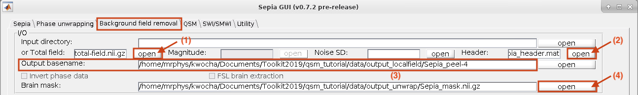
In the I/O panel, specify the required files by using the open buttons in the second row:
Total field: Sepia_total-field.nii.gz (from the output directory of the previous exercise),
Header: Sepia_header.mat (from the input directory),
Change the Output basename to: ~/qsm_tutorial/data/output_localfield/Sepia_peel-4
Brain mask Sepia_mask.nii.gz (from the output directory of the previous exercise, which will tell the software what is not part of the background.)
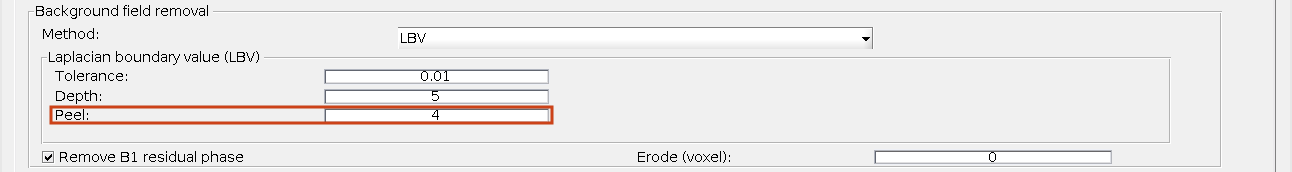
Second, in the Background field removal panel, the ‘LBV’ method is shown by default. You can have three parameters to adjust.
‘Tolerance’: a threshold to stop the algorithm.
‘Depth’: multigrid level.
‘Peel’: the layer of boundary voxels to be removed after computing the tissue (or so-called local) fields.
Set Peel to: 4
Press the Start button.
Again, when the process is finished, you will see the message: ‘Processing pipeline is completed!’.
Use FSLView to display the local field map (Hz) (should be in ~/qsm_tutorial/data/output_localfield/).
fslview_deprecated Sepia_peel-4_local-field.nii.gz &Adjust the display window to ‘Min -5’ and ‘Max 5’.
Note you can clearly see the contrast between grey and white matter, and veins and tissue now. Other structures as the globus pallidus, red nuclei and substantia nigra are visible… but not quite normal.
Compare the location of the edges of brain structures with what you can see in the mean magnitude image computed in Exercise 1.
Use shortcut
Crtl+Ain the FSLView to add mean_head.nii.gz to the displayed local field maps.Adjust the display window of mean_head.nii.gz to ‘Min 0’ and ‘Max 300’.
Go to location [133 155 81] which is on the top edge of the globus pallidus.
Check/Uncheck the ‘Visibility’ button to turn on/off of the mean magnitude image.

It is known that there is a high concentration of iron deposition in the globus pallidus. There it generated a strong secondary magnetic field. Can you identify the magnetic field generated by this structure?
You can close all the FSLView window(s) now.
Proceed to Exercise 4.
Advanced Exercise 3.2
Note
If you still have enough time, follow the exercise below.
In this exercise, we will focus on the differences of using different ‘Peel’ values.
Change the Output basename to: ~/qsm_tutorial/data/output_localfield/Sepia_peel-2
Set Peel to: 2
Press the Start button. Again, when the process is finished, you will see the message: ‘Processing pipeline is completed!’.
Use FSLView to display the local field map (Hz) when using ‘Peel’ value of 2 (should be in ~/qsm_tutorial/data/output_localfield/):
fslview_deprecated Sepia_peel-2_local-field.nii.gz &Load the Sepia_peel-4_local-field.nii.gz map in the same window. You can do this by selecting ‘File → Add…’ (or shorcut
Crtl+A) and select Sepia_peel-4_local-field.nii.gz in the window provided.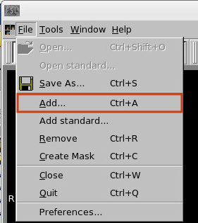
Adjust the display window to ‘Min -5’ and ‘Max 5’ for both images.
Set location as [119 142 88]. Look at the differences between the two maps globally.
Check/Uncheck the ‘Visibility’ button in the bottom of the viewer to turn on/off of the top image. What are the main differences between the two results?
Proceed to Exercise 4.
Back to Exercise 2.